Visual Pipeline Editor

megane's pipeline editor lets you build visualization workflows by wiring nodes — no code required. Open the pipeline panel from the sidebar to start building.

The visual pipeline editor: nodes on the canvas, live 3D on the right.

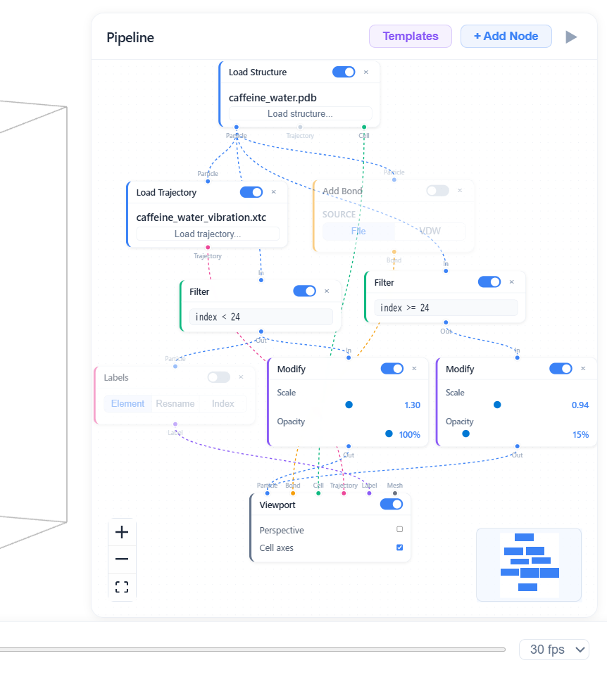
Pipelines can also be built programmatically in Python, TypeScript, or written directly as JSON.

For real-world examples, see the Gallery.

Concept

A pipeline is a directed graph of nodes connected by edges. Data flows from source nodes (like Load Structure) through processing nodes (like Filter or Modify) and into a Viewport node for rendering.

Each edge carries a specific data type — particle, bond, cell, label, mesh, trajectory, vector, or volumetric — and only matching types can connect.

When a node encounters an error — for example, a parse failure in LoadStructure — an error icon appears on the node with a tooltip showing the details.

AI Pipeline Generator

Describe the visualization you want in natural language, and megane builds the node graph for you. Open the AI chat panel from the pipeline editor toolbar and type a prompt like:

Load protein.pdb with bonds and make water translucent

The generator creates the appropriate LoadStructure, AddBond, Filter, Modify, and Viewport nodes, wires them together, and places them in the editor. You can then adjust parameters or add more nodes manually.

VS Code Extension Auto-Setup

When you open a supported molecular file (.pdb, .gro, .xyz, .mol, .sdf, .mol2, .cif, .mmcif, .data, .lammps, .prmtop, .traj, .xtc, .dcd, .lammpstrj, .dump, .nc) in the megane VS Code extension, it automatically creates a default pipeline consisting of LoadStructure → AddBond → Viewport. This gives you an immediate 3D view of the structure with bonds, without needing to build a pipeline manually. You can then modify the auto-generated pipeline in the editor as needed.

Getting Started

The simplest pipeline loads a structure and displays it:

LoadStructure → Viewport

To add bonds inferred from atomic distances:

LoadStructure → AddBond → Viewport
                       ↘
              LoadStructure → Viewport (particle + cell)

Use the Templates dropdown to load pre-built pipelines:

• Molecule — Caffeine (caffeine_water.pdb) with structure-based bonds and a vibration trajectory (caffeine_water_vibration.xtc). Nodes: LoadStructure → Wrap → AddBond → Viewport, LoadTrajectory → Wrap → Viewport.
• Molecular Crystal — Glycine (glycine_csd.cif) with atoms normalized into the home cell and finite molecules completed across its faces. Nodes: LoadStructure → Wrap, followed by parallel AddBond and DrawingBoundary branches that join at BoundaryCompletion → Viewport.
• Solid — Perovskite SrTiO₃ 3×3×3 supercell with TiO₆ coordination polyhedra. Nodes: LoadStructure → Wrap → DrawingBoundary → Coordination → PolyhedronGenerator → Viewport. Coordination detects metal centers and neighboring anion-former atoms; its Bond output also renders the neighbor atoms required to complete boundary coordination environments.
• ESP Isosurface — Caffeine (caffeine.sdf) overlaid with its electrostatic potential read from a cube file (caffeine_esp.cube). Nodes: LoadStructure → Symmetry → Wrap → AddBond → Viewport alongside an independent LoadVolumetric → Isosurface → Viewport (mesh) branch. The two branches never meet in the graph — the molecule and the grid line up because they share a coordinate frame. The Isosurface node runs in dual-contour mode (showNegative), so it draws the potential at both +isoLevel (blue, over the methyl and imidazole hydrogens) and −isoLevel (red, over the two carbonyl oxygens), the usual chemistry convention. The default level, 0.03 Hartree/e, is where the potential sits on caffeine's van der Waals surface; lower it in the node to grow the lobes into a shell around the whole molecule.
• Coarse-Grained Overlay — Ubiquitin before and after coarse-graining, superimposed: the all-atom model (1ubq.pdb) ghosted at 30 % opacity behind one bead per residue (1ubq_cg.pdb, each bead at its residue's heavy-atom center of mass). Two LoadStructure nodes feed one Viewport and render as separate structure layers. The all-atom side splits into two Filter → Modify branches — protein at opacity 0.3, the 58 crystallographic waters at opacity 0 — because a Modify behind a Filter writes its opacity only at the selected atoms and leaves the rest fully opaque. The bead side scales up ×3.2 and takes a uniform Color so it reads over the ghost, with its backbone drawn from the CG file's CONECT records.

Molecule template — caffeine in water

Solid template — SrTiO₃ supercell

Node Reference

Every node type — its purpose, ports, and every parameter — lives in the Node Reference, generated directly from the pipeline source (src/pipeline/catalog.ts) so it never drifts from the code. Jump straight to a node, e.g. polyhedron_generator.

Data Types

Nine typed data channels flow through color-coded edges:

Type	Color	Description
particle	Blue	Atom positions, elements, and optional indices/overrides
bond	Amber	Bond pairs and orders
cell	Emerald	Simulation cell (3×3 matrix)
label	Violet	Text labels positioned at atoms
mesh	Gray	Triangle mesh for polyhedra rendering
trajectory	Pink	Multi-frame coordinate data
vector	Red	Per-atom 3D vector data (forces, velocities, etc.)
volumetric	Cyan	Scalar field on a 3D grid, consumed by the Isosurface node
spectrum	Lime	2D (x, y) trace, consumed by the terminal Spectrum Plot node

Filter DSL

The Filter node accepts Python-like query expressions to select atoms.

Available Fields

Field	Type	Description
element	string	Element symbol (e.g., "C", "O", "Fe")
index	number	Atom index (0-based)
x, y, z	number	Cartesian coordinates
resname	string	Residue name (e.g., "ALA", "HOH")
mass	number	Atomic mass
molecule_id	number	0-based connected-component (molecule) ID, derived from bond connectivity. Atoms with no bonds form their own single-atom molecule

Operators

==, !=, >, <, >=, <=

Logical Operators

and, or, not, parentheses ()

Special Keywords

all — select all atoms, none — select no atoms

Examples

element == "C"                         # All carbon atoms
index > 10 and index < 20             # Atoms 10–19
resname == "HOH"                       # Water molecules
not element == "H"                     # Non-hydrogen atoms
element == "O" or element == "N"       # Oxygen or nitrogen
(x > 0 and x < 10) and element == "C" # Carbons in x range
mass > 32                              # Atoms heavier than sulfur
molecule_id == 0                       # Atoms belonging to the first molecule
not molecule_id == 0                   # Everything except the first molecule

Bond Selection DSL

The Bond query field in the Filter node accepts expressions to select bonds.

Available Fields

Field	Type	Description
bond_index	number	0-based sequential bond index
atom_index	number	Atom endpoint index
element	string	Element symbol of an atom endpoint (e.g., "C", "O")
molecule_id	number	0-based molecule ID of the bond's endpoints (both endpoints always share the same ID)

Operators

==, !=, >, <, >=, <=

Logical Operators

and, or, not, parentheses ()

Special Keywords

• all — select all bonds (default when query is empty)
• none — select no bonds
• both — prefix on a comparison involving atom_index or element to require both atoms of the bond to satisfy the condition (default: either atom, OR semantics). Has no effect on bond_index comparisons, and is redundant (but harmless) for molecule_id, since both endpoints of a bond always share the same molecule ID.

Examples

element == "C"                         # Bonds where either atom is carbon
both element != "H"                    # Bonds where neither atom is hydrogen
atom_index >= 24                       # Bonds involving atom 24 or higher
bond_index < 10                        # First 10 bonds only
both atom_index >= 0 and bond_index < 50  # First 50 bonds (all-atom filter)
molecule_id == 0                       # Bonds within the first molecule

The bond query selects which bonds a downstream Modify node applies opacity overrides to. This lets you selectively fade specific bonds without removing them from the scene.

Editor Examples

TiO₆ Octahedra in SrTiO₃

1. Load a perovskite structure (LoadStructure)
2. Add a PolyhedronGenerator node
3. In "Excluded centers", add Sr (38) so only TiO₆ polyhedra are shown (Ti and O are auto-detected)
4. Connect LoadStructure.particle → PolyhedronGenerator.particle
5. Connect PolyhedronGenerator.mesh → Viewport.mesh

Or use the Solid template which sets this up automatically.

Make Solvent Translucent

Use Filter + Modify nodes to fade out water molecules while keeping the protein fully visible.

1. Add a LoadStructure node and load your PDB file
2. Add a Filter node with query: resname == "HOH"
3. Add a Modify node and set opacity to 0.2, scale to 0.5
4. Connect: LoadStructure.particle → Filter.in → Modify.in → Viewport.particle
5. Connect the original LoadStructure.particle → Viewport.particle as well (for the protein)

The viewport renders both streams — the protein at full opacity, and the water as translucent small spheres.

Modify a Single Molecule (Atoms + Bonds Together)

molecule_id lets you target one molecule (a connected component of the bond graph) and fade its atoms and bonds together, using the same query on both streams.

1. Add a LoadStructure node and load a structure with multiple molecules (e.g. caffeine_water.pdb)
2. Add an AddBond node and connect LoadStructure.particle → AddBond.particle to produce a bond stream
3. Add two Filter nodes:
   • Filter A (atoms): query not molecule_id == 0
   • Filter B (bonds): bond query not molecule_id == 0
4. Add two Modify nodes and set opacity to 0.15 on each
5. Connect:
   • LoadStructure.particle → FilterA.in → ModifyA.in → Viewport.particle
   • AddBond.bond → FilterB.in → ModifyB.in → Viewport.bond
   • LoadStructure.particle → Viewport.particle and AddBond.bond → Viewport.bond (original full-opacity streams)

Molecule 0 (the component containing atom 0) stays fully opaque, while every other molecule's atoms and bonds fade together — both Filter nodes derive molecule_id from the same underlying bond connectivity.

Expand a Crystal's Asymmetric Unit

A CIF lists only the crystallographic asymmetric unit plus the space-group operations, and megane's parser returns exactly that. The Symmetry node applies those operations to fill one unit cell with the symmetry-equivalent molecules, VESTA-style. Every default pipeline and structure template already carries one directly after LoadStructure in its expand mode, so a loaded CIF shows the full unit cell out of the box:

1. Load a CIF (other formats carry no space-group operations, so the node is a transparent pass-through for them)
2. Select the Symmetry node in the graph
3. Pick a mode:
   • Expand applies the space-group operations (the default) — bonds are replicated per symmetry image, and images that coincide on special positions are dropped
   • None shows the raw asymmetric unit exactly as the file lists it

Pipelines saved before the node existed have no Symmetry node, so a CIF loaded through them shows the asymmetric unit; add the node after LoadStructure to recover the packed cell.

Wrap / Unwrap a Periodic Structure

The Wrap / Unwrap node toggles periodic-image coordinate mapping without changing the file. Every default pipeline and structure template already carries one between LoadStructure and the rest of the graph in its pass-through mode (none), so the toggle is a single dropdown click:

1. Load a periodic structure (a unit cell is required)
2. Select the Wrap / Unwrap node in the graph
3. Pick a mode:
   • Wrap folds every atom back into the home unit cell (useful for trajectories whose coordinates drift out of the box)
   • Unwrap shifts atoms by whole lattice vectors so molecules split across a periodic face become whole again, VESTA/Mercury-style — connectivity comes from the file's bonds, or the same distance-based inference the AddBond node uses when the file has none
   • None passes coordinates through untouched (the default)

A connected trajectory is remapped frame by frame with the same convention, so playback follows the chosen mapping too. The unit cell itself never changes — unwrapped molecules may poke outside the cell wireframe.

Multiple Structure Layers

You can load multiple structure files simultaneously, with each file rendered as a separate layer in the viewport. Each LoadStructure node connected to a Viewport creates an independent rendering layer, allowing you to combine different molecules in a single view.

For example, to display a protein and a ligand loaded from separate files:

LoadStructure (protein.pdb) → AddBond → Viewport
LoadStructure (ligand.mol)  → AddBond ↗

Each layer is processed independently through its own chain of Filter, Modify, and overlay nodes before reaching the Viewport.

---

For more examples with code, see the Gallery.